Free space EM solvers are essential tools for calculating electromagnetic fields in various environments. These solvers use numerical methods to simulate the behavior of electromagnetic waves and fields, providing valuable insights for engineers and researchers. In this article, we will explore the key aspects of free space EM solver field calculation, highlighting the most critical factors to consider when working with these powerful tools.
1. Understanding the Basics of Electromagnetic Fields
Before diving into the world of free space EM solvers, it's essential to understand the fundamentals of electromagnetic fields. This includes knowing the different types of electromagnetic waves, such as radio waves, microwaves, and light, as well as the concepts of frequency, wavelength, and amplitude. A solid grasp of these basics is crucial for effectively using free space EM solvers and interpreting the results.
2. Choosing the Right Numerical Method
Free space EM solvers employ various numerical methods to calculate electromagnetic fields, including the Finite Difference Time Domain (FDTD) method, the Method of Moments (MoM), and the Finite Element Method (FEM). Each method has its strengths and weaknesses, and selecting the right one depends on the specific problem being solved. For example, FDTD is well-suited for simulations involving complex geometries, while MoM is often used for problems with large domains.
3. Defining the Simulation Domain
The simulation domain is a critical aspect of free space EM solver field calculation. It defines the region where the electromagnetic fields will be calculated, and its size and shape can significantly impact the accuracy and computational efficiency of the simulation. The domain should be large enough to encompass the entire region of interest, but not so large that it becomes computationally prohibitive.
4. Discretizing the Simulation Domain
Once the simulation domain is defined, it must be discretized into smaller cells or elements. This process, known as meshing, allows the numerical method to approximate the electromagnetic fields at each point in the domain. The mesh size and quality can significantly impact the accuracy of the simulation, and different meshing techniques, such as uniform and non-uniform meshing, can be used to optimize the calculation.
5. Applying Boundary Conditions
Boundary conditions play a crucial role in free space EM solver field calculation, as they define how the electromagnetic fields behave at the edges of the simulation domain. Common boundary conditions include perfect electric conductors (PEC), perfect magnetic conductors (PMC), and absorbing boundary conditions (ABC). Each boundary condition has its own set of assumptions and limitations, and selecting the right one depends on the specific problem being solved.
6. Including Material Properties
In many cases, the simulation domain will include different materials with varying electromagnetic properties, such as permittivity, permeability, and conductivity. These properties must be accurately modeled in the simulation to ensure realistic results. Free space EM solvers often include libraries of common materials, and users can also define custom materials with specific properties.
7. Exciting the Simulation with Sources
To calculate the electromagnetic fields, the simulation must be excited with a source, such as a plane wave, a point source, or a antenna. The source defines the type and intensity of the electromagnetic radiation, and its placement and orientation can significantly impact the results. Users can often choose from a range of built-in sources or define custom sources to match their specific needs.
8. Visualizing and Analyzing the Results
Once the simulation is complete, the results must be visualized and analyzed to extract meaningful information. Free space EM solvers often include powerful visualization tools, such as 2D and 3D plots, animations, and charts, to help users understand the behavior of the electromagnetic fields. Users can also perform various analyses, such as calculating field strengths, power densities, and scattering parameters, to gain deeper insights into the simulation results.
9. Validating the Simulation Results
To ensure the accuracy and reliability of the simulation results, it's essential to validate them against analytical solutions, measurements, or other numerical methods. This involves comparing the simulation results with known values or trends to verify that the solver is producing correct and consistent results. Validation is a critical step in building trust in the simulation results and ensuring that they can be used for making informed design decisions.
10. Optimizing the Simulation Performance
Finally, optimizing the simulation performance is crucial for efficient and effective use of free space EM solvers. This involves selecting the right numerical method, mesh size, and simulation parameters to achieve the desired balance between accuracy and computational efficiency. Users can also leverage advanced techniques, such as parallel processing and GPU acceleration, to speed up the simulation and reduce the overall computation time.
If you are searching about EM Solver Technology – Lorentz Solution you've came to the right page. We have 10 Images about EM Solver Technology – Lorentz Solution like EM Solver Technology – Lorentz Solution, Schematic view of the near-field solver and the far-field solver for and also Representation of the calculation field with its dimensions, and the. Here you go:
EM Solver Technology – Lorentz Solution
 www.lorentzsolution.com
EM Solver Technology – Lorentz Solution
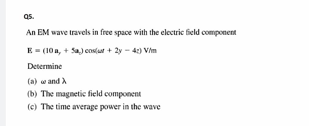
Solved An EM Wave Travels In Free Space With The Electric | Chegg.com
 www.chegg.com
Solved An EM wave travels in free space with the electric | Chegg.com
2-D Field Solver - MATLAB & Simulink
 www.mathworks.com
2-D Field Solver - MATLAB & Simulink
Schematic View Of The Near-field Solver And The Far-field Solver For
 www.researchgate.net
Schematic view of the near-field solver and the far-field solver for ...
Solver Settings For The Determination Of The Velocity Field | Download
 www.researchgate.net
Solver settings for the determination of the velocity field | Download ...
Solved An EM Wave Travels In Free Space With The Electric | Chegg.com
 www.chegg.com
Solved An EM wave travels in free space with the electric | Chegg.com
2: Boundary Conditions For Field Solver, And How They Are Applied To
2: Boundary conditions for field solver, and how they are applied to ...
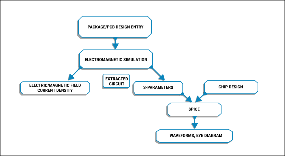
Significance Of Electromagnetic Field Solvers | Sierra Circuits
 www.protoexpress.com
Significance of Electromagnetic Field Solvers | Sierra Circuits
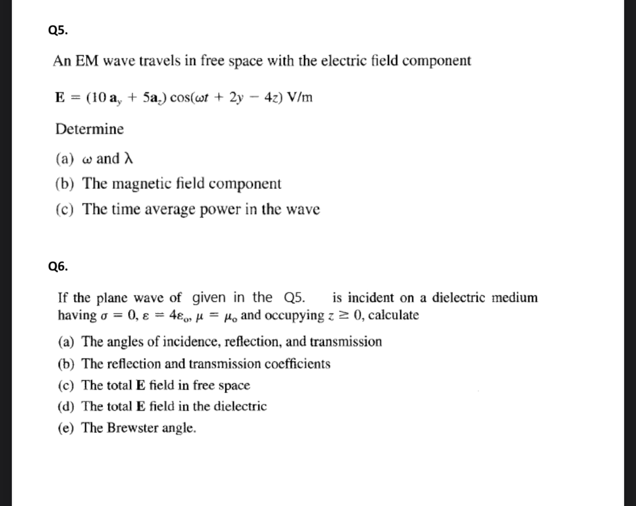
Solved Q5.An EM Wave Travels In Free Space With The Electric | Chegg.com
 www.chegg.com
Solved Q5.An EM wave travels in free space with the electric | Chegg.com
Representation Of The Calculation Field With Its Dimensions, And The
 www.researchgate.net
Representation of the calculation field with its dimensions, and the ...
Em solver technology – lorentz solution. Solved an em wave travels in free space with the electric. em solver technology – lorentz solution

